
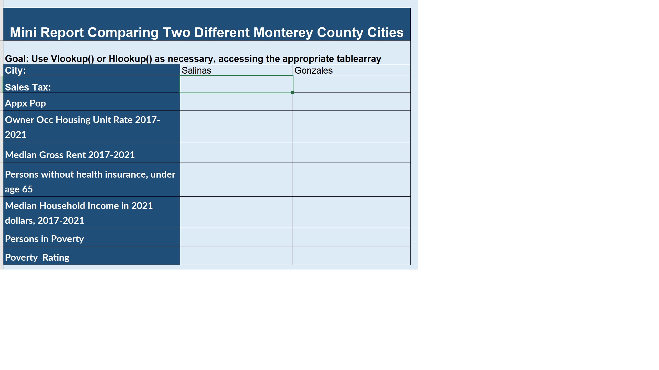
So, to complete this report, we are going to use three different tables of information, and we’re going to need to use Vlookup() with an EXACT match, and Vlookup() with a RANGE match. And we’re going to use Hlookup() with an EXACT match. The first row in this table, below the city names, is Sales Tax, and we have a table of Sales Tax information for Monterey County cities on a worksheet entitled Sales Tax Monterey County. And we can take a look at the Table Array
by choosing the name of it from the name box in the left corner, and we see that the city names are in the vertical column, to the far left, and the tax rate is in column 2 in relation to the first column. So we’re going to do an EXACT match lookup to find the tax rate, the Sales Tax rate of those two different cities.
The Lookup Value will be the name of the city.
The Sales Tax Table Array will be the Table Array, the Column Index to return once the match is found will be column 2, and we definitely want an EXACT match to our city name, so we’re putting FALSE.
Because we use a relative reference for our city name, we can drag this to the right and use the same formula for the second city in the table. Now to find the next one, two, three, four, five, six values in this table, we’re going to pull from a City Demographics Table that was gathered from Census Data from 2021. And in this Table Array,
the names to match are arranged in a row instead of a column, and we’re not going to take every value from this. We’re going to take different ones, depending on what the report asks for, but we’ll need to provide Row Index Numbers and the first value we’ll be looking for is Approximate Population, which is in row 2, the first row below the row in which a match needs to be found. So let’s go back to the report.
This is an Hlookup().
Lookup Value is again the city,
but this time I’m thinking about how I’m going to use the same formula for several rows of this report, and I like to be able to copy it where I can, and then just change what I need to change. And I’m going to use the same cities for lookup in each of the rows of this report, so I if I have a RELATIVE reference and I copy this to a new row, the row is going to change, the Row Number of that City Name, and I don’t want it to. So, I’m going to make my cell reference, referencing the city to look up in the table, into an ABSOLUTE reference, but then change it to be a MIXED reference. I’ve changed it so the COLUMN can change when I copy to the right for a different city, but the ROW can’t change when I copy it down to look up a different value.
Now the Table Array I want, is the City Demo Table Array.
And I already noted that the Row Index for Approximate Population is row 2 of that table, and I definitely am looking for an EXACT match to my city name.
So my Approximate Population, I’m going to format that to look
like a number with a comma between the thousands place.
And I’m just double checking that my formula here looks correct: it’s referencing the city of Gonzales in C4 and the same table array Row 2, EXACT match.
Now,
I can drag this down and I get the same results because I’m still looking up the same Approximate Population, but I want to change the formula so that I’m looking up Owner Occupied Housing Unit Rate, which is in Row 3 of that table,
and that’s a percent, and I’ve got this formatted as a number, so I need to increase my decimal places so I can see the the values of the percent, and then I’m going to change it to percent format. Now I’m going to copy that to the right and get the correct value for the second city as well.
I’m just gonna copy down the one in the first column for Median Gross Rent, because I know I’m going to have to change the formatting after I change the Row Index. So again, I’m going to change my Row Index for Median Gross Rent, and that is 5
from that table, and then I’m going to change it to a $ symbol,
and let’s reduce the zeros, and drag that over.
Now we want to get the Percent of Persons Without Health insurance Under the Age of 65. That value is in row 6.
Let’s add a decimal place.
The Median Household Income is in row 8.
Change that back to dollars,
and get rid of extra zeros.
Then the Percent of Persons in Poverty is in row 9.
Change that to a percent,
add some decimal places,
and drag it across. Now this last one is a Poverty Rating, where we’re comparing it to the Percent of Persons in Poverty in the U.S, as a whole. And we’ve got a Table, a very small table, set up for this Poverty Level Table Array. It just has two entries, either the rating is “Below the U.S persons in Poverty Percent” or it’s “Greater than or Equal,” because the
overall Percent of Persons in Poverty in the U.S, as a whole, according to the 2021 census, was 11.6%. So we’re going to go ahead and use this Povlev Table Array and we’re going to do a RANGE Vlookup() this time.
A RANGE lookup. So, doing Vlookup(),
and we’re looking up the Percent of Persons in Poverty this time, NOT the CITY. We want, we’re looking at the value that resulted from that Look Up for the Percent of Persons in Poverty, and we’re going to look in the Poverty Level Table Array,
and we want the second column contents as our result to our function. And this time we’re looking for a RANGE match. So we’re gonna, we could omit that fourth argument and the default would be TRUE but we’re going to make it explicit, just to make the point.
And here we get “Greater Than or Equal to U.S Persons in Poverty Percent.” Now let’s drag this across and we see that this is “Below US Persons in Poverty Percent.” And we can make this a little more readable by expanding this row a little bit and wrapping the text
so that it fits into that cell.
And that is, let’s see we can take a quick look at
the formulas in here, but I’m not going to do that for this. I’m going to say “Thank you very much, see you in another video.”