
We’re going to jump to the Nested If and Range Lookups worksheet and adjust the page so you have the optimal view.
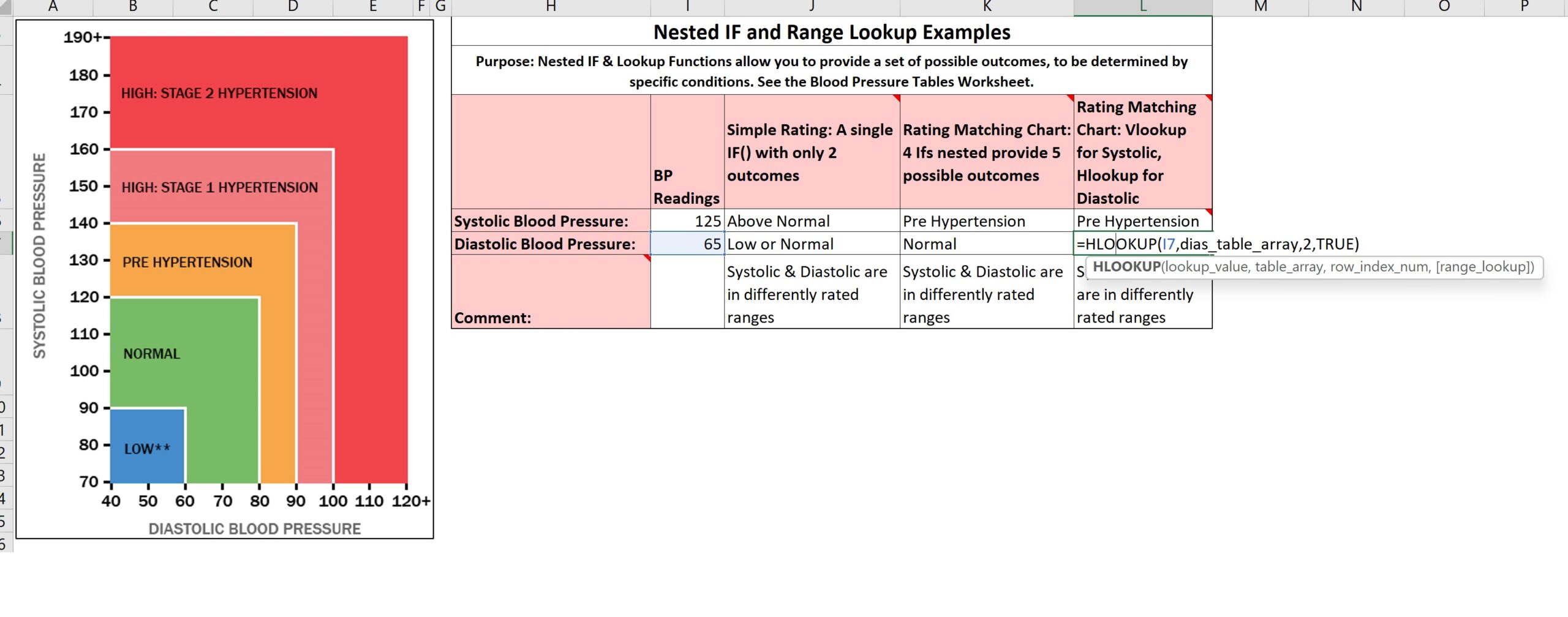
This is an example where we have a table that includes two blood pressure readings: a Systolic reading and a Diastolic reading. And we can see on this chart to our left that the Diastolic blood pressures are on the x-axis horizontally, and the Systolic are on the y-axis vertically. And we’ve emulated this table by creating blood pressure table arrays. We’ve got a Diastolic blood pressure table array that’s arranged horizontally with the lowest possible reading in the top left corner, and then the readings move across that top row horizontally to the highest indicator that’s included in the table. So the way that this table is meant to be understood, a reading of anything 0 or less than 60 would fall into the “low” range. Anything 60 but less than 80 would fall in the “normal” range. Anything greater than or equal to 80 but less than 90 would fall in the “pre-hypertension” range, and anything greater than or equal to 90 but less than 100 would fall into the “stage one hypertension.” Anything greater than 100 on up to as high as it could be, will, using the results of this table, just indicate “stage 2 hypertension.” It could be that the table could go on further, but this is the limits of the table we’ve designed here, and we’ve named this table Dias Table Array for Diastolic blood pressure. And it’s arranged with, the idea is, to be able to use it for an Hlookup(), a horizontal lookup. So back to the table where we have this diastolic blood pressure reading of 65,
if we look into this contents of cell L7, we see an Hlookup() Function. The Lookup Value is in I7, which is 65. And the table to look in for a match, a RANGE match, is Dias Table Array. And once the match is found, we’re asking Hlookup() to return the value in row 2 of that table, from the same column in which the match for I7 was found. And the TRUE value of the Range Lookup argument tells Excel that we want a RANGE match, not an EXACT match. So the way Excel will operate, it’ll take this value I7, which happens to be 65. It’ll go to that Dias Table Array and it’ll start in this top left corner. It’ll say, “Is that 65 greater than or equal to zero?” If yes, it’ll go on to the next, (actually, am I misremembering? is that 65? yes, okay)
it’ll go on to the next
value in this horizontal row, the top row of this Table Array. It says, “Is 65 greater than or equal to 60?” and the answer is yes, so it could be in this range. So then it goes on to the next column in that top row. It says, “Is 65 greater than or equal to 80?” No, it’s not. It’s less than 80. So it falls back here. It says, “This is the range that my Lookup Value falls within.” So now I’m going to return the value in row 2 of the same column of the Table Array that I found my RANGE match, and that value is “normal.” So we go back to our table indicating the rating for this blood pressure reading, we see that we did get the result “normal” for that reading.
Thank you very much.