
Welcome to excel intuition, I’m Suzanne. This module looks at lookup functions. We’re going to look at two different lookup functions: VLOOKUP, for looking things up in a vertical column, HLOOKUP for looking things up in a horizontal row.
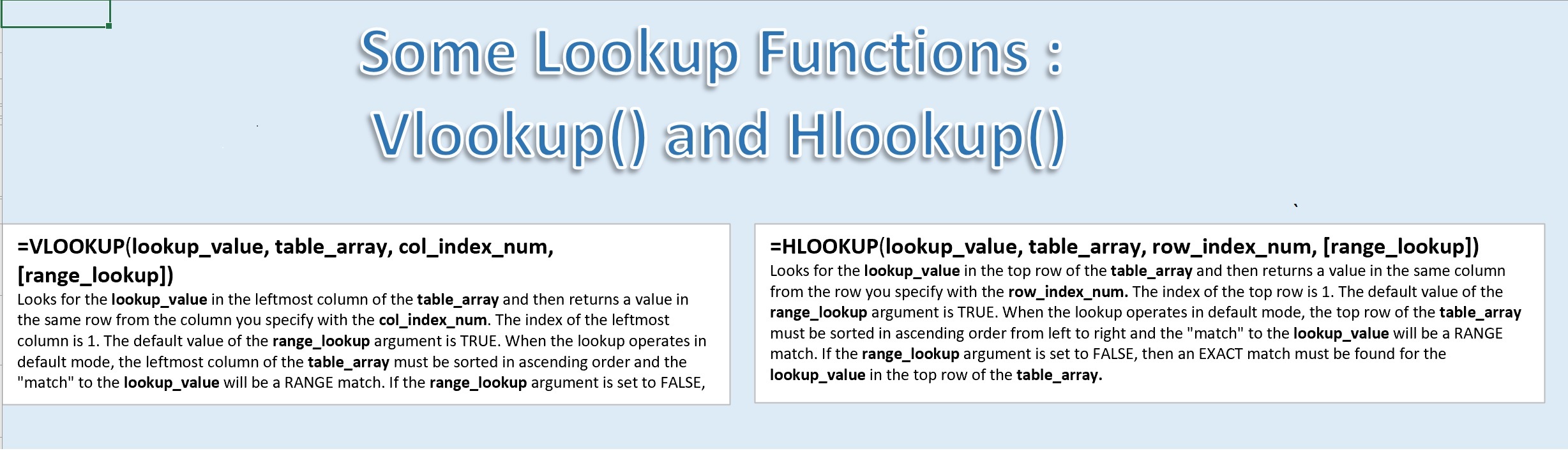
Both VLOOKUP and HLOOKUP have the same number of arguments. The first argument is the lookup_value that you want to look up in the table_array, which is the second argument. And then there is an index number as a third argument to each function. It’s a column index number in the VLOOKUP and a row index number in the HLOOKUP, so the idea is when you find the look up value in the column of the table array for a VLOOKUP, you’re looking in the very first column of the table array. You’re always looking in the left most column for a match. Once you find it, you’ll be in a specific row of the table array, and the column index number tells you which column of that row you want the value returned from, as the result of the functions look up. The range_lookup argument is an optional argument, and if you don’t use it, it defaults to a value of true. And that means you aren’t looking for an exact match to your look up, you’re looking for a range match.
With HLOOKUP, we’ve got the look up value is the first argument, the table array is the second, but in this case the table array is arranged so that we’ll be looking for the look up value in the top row of the table, and when we find the value in a particular column in that top row, then the row index number says which row of that column we want the value returned from. The range look up argument works the same way here, that if we don’t use it, it defaults to true, and then we want a range look up instead of an exact match look up. If the range_lookup argument is set to false we want an exact match in our look up. And we’re going to see an example of exact match look ups, and then we’ll see one example of a range look up.
So in the first example, we have two cities in a mini report, and we want to look up their sales tax rate for the cities. And the table that we have for the sales tax rates, is a vertical table in that cities are the city names are in a vertical column. So once you find a match to a name you see the sales tax rate is in column two of the same table. So the VLOOKUP argument here uses as it’s first argument, the lookup_value is the city name that we see in B7, the salestax_table_array is the second argument, and we see that we’re telling it to give us the value from column 2 of that table. The range_lookup argument is false, meaning we want an exact match look up. We’re not going to get an answer from this function if there isn’t a name that exactly matches the name Salinas in that table. So if we have this set up so that you can choose the name from a drop down list. So you really don’t have the possibility of entering your name that there won’t be a match for.
If we go to the sales tax table, you can see the range that has been defined for the table array, if you choose that named range from that name box. And we can see it’s C4 down to E13. And if we choose a different name from this list, we’ll get a different tax rate.
Now in the HLOOKUP example, we’re looking up a value from a different table, we’ve got the same lay out of two different city names, but we’re looking up a percent of persons in poverty in these cities according to the us census data gathered. So that table is on this worksheet called city demographics. And we see that our city names are organised in a row instead of a column, and then the data associated with them is in the rows below that. And the row that we’re looking a value up from is all the way at the bottom of the table in row 9 of the table. The percent of persons in poverty according to the US census data. And there’s a link to the web page that has that data available if you’d like to look at it further. I’m going to show you the table array here also, it’s the citydemo_table_array and you can see it does not include the the column with the names of the values in the rows, it includes D3, where the city names start, over to M11. Those are the rows in this table array. So our HLOOKUP function, the lookup_value is the city name again. The citydemo_table_array is that table array that i just showed you, and then the row that has the persons in poverty value that we want returned once we find a match to the lookup_value is row 9. The false indicates that we must find an exact match. If there wasn’t an exact match this function would return an error.
Now I have another look up example here where we’ll use a range look up for a VLOOKUP. In this case I have a little report that we’re asking to have a poverty rating displayed here. A message that says whether the city in this column has persons in poverty percent value less than the us overall percent of persons in poverty, or greater than or equal to the us persons in poverty percent. Let me go back to the city demographics table and show you that value. We’ve got values for cities in Monterey County with a population over 5000 in this table, but then we have values for the US as a whole in this column on the left. And that persons in poverty percent is at the bottom of the column. 11.6 was the percent according to the US census from 2017 to 2021. That’s the percent of persons in poverty in the US as a whole. So on this example we want to compare the percent of persons in poverty in the city in this column to the percent of persons in poverty in the US as a whole.
So we’ve got a table over here that has zero at the bottom and 11.6 as the second value in the table. This is organised vertically, the value zero and the value of US persons in poverty percent and there’s a comment here that explains what it is as well. So the way a range look up works, you take a value to a table and you compare it one by one to the values in the column, or the row if it was an HLOOKUP, and you say is this value greater than or equal to this value. If it’s not, your table wouldn’t… if the the value you’re taking to the look up is not greater than or equal to the first value in the table, it would have an immediate error because the table wouldn’t be set up properly. For a range look up the table has to be an ascending order, and the first value has to be less than or equal to the value you want to find a look at match for.
So the way VLOOKUP with the range match works, it compares with the first value says is it greater than a equal? And if that’s true it continues on and it looks to the second value and says is it greater than our equal? In this case it would be true that it was greater than our equal to 0, and it would be true that it was greater than or equal to 11.6. And there’s no further entries in this table so it would stop here and this would be the message. Greater than or equal to US persons in poverty percent, and that’s the message that we see right here. Now in the second column, with the same look up process, we take this value, is it greater than equal to 0? Yes. Is it greater than or equal to 11.6? No. So it stops here, and this would be the message returned from column 2. And we can see that there’s three arguments here, the lookup_value, the table_array, which is these 4 cells, and then 2 is the column to return a value from once the range match is found.
So now we’re going to apply these different look ups to a new little report, and I recommend if you haven’t already done so you download your own copy of this companion file and try this on your own before watching the demonstration of the solutions. So here we have again two different cities to be compared with each other, you can choose from a drop down list different names for the columns, as you wish. I’m trying to… okay. And then the first value we want to compare is their sales tax rates, and we know that the sales tax on this table, and that it’s a vertical table, and we know the name of the table, salestax_tablearray. So in this report we’re going to make a VLOOKUP function, looking up the name of the city. And since we know the name of the table array we can start typing it, if i just type an “S” I’ll get choices that start with “S” to choose from, and I can just double click on this table array to put it into my formula. Then I also remember that the sale tax rate is in column two of the table, once the name of the city is found, and i want an exact match. I don’t want a city named close to the name of the city i’m looking at, I want it to be exactly the name I’m looking for. So i’m putting false for the range_lookup argument. And i can drag this to this column, because the the reference to B4 is going to change to C4 because it’s a relative reference, and when i moved the formula it will change relative to being in a new column.
Now the approximate population value is in a different table array, it’s not in the salestax_tablearray. Now i’m going to be looking things up in the city demographics table array and that’s a horizontal look up because the city names are arranged in a horizontal row at the top of the table. And I see that the population estimates are in row 2 of the table. So i’m going to use my HLOOKUP and my lookup_value is again city, but this time I’m noticing that a number of values are going to come from the same table and use the same lookup_value and i’d like to be able to create a formula i could drag down this column and just change the row index number, not have to create the formula from scratch. If i want to do that I need to change this reference to the lookup_value to be a mixed reference instead of a completely relative reference because I don’t want the row of the reference to change when I drag it down, I still want to column to change when i drag it to the right. So if i click my F4 key that would be an absolute reference which wouldn’t change at all but then it wouldn’t change to C4 when I move it to the right. So I’m going to make a mixed reference, the dollar sign in front of the 4 means that will not change but the B will be allowed to change if the relative reference, if the formula moves to a new location. The table array I want is the city demo table array, and for the population I want values from the second row so I’m using two as my row index and again I want an exact match. And i could formulate this to look like a number, with a comma, and I don’t need those extra decimal places.
Now the next value I want is owner occupied housing unit rate, what percent of housing is occupied by owners of those houses in these cities. Now I copied this straight down, I had to change my index number to the correct row and that is row 3, and then I’m going to want to change my formatting, because this needs to be formatted as a percent not as a whole number and I’m going to add a little decimal place there.
Now I’m going to drag this down again, this time I want the median gross rent, which is in row 5. So I’m going to change the 3 to a 5. And change it from a percent to a dollar value, take away the decimal places this time. Here the value, this is a percent value again, this person’s without health insurance, so I’m going to copy the formula from where I already have it formatted as a percent to make this transition smoother. And this is coming from row 6, so I change my row index from 3 to 6. And this is the percent of persons without health insurance under the age of 65 in this town of Pacific Grove.
Now the next value I want is the median household income in 2021 dollars from the census period of 2017 to 2021, so I’m going to copy the formula from one that I’ve already formatted as dollars, and then change my row index to eight, which is the row where that information is stored.
And then the persons in poverty is also a percent, so i’m going to copy from a percent formatted cell, but change my row index to 9 because that’s row 9 of the table where that value’s stored.
And then the rating I’m going to get from the same table that we had it when we had this example of the range look up. So I’m comparing here this percent to the US percent of persons in poverty, so I’m going to use a VLOOKUP, my lookup_value is this percent. I’m going to do a relative… I’m going to just leave it as is, because I’m only going to copy it over to the cell to the right, so I don’t have to make it a mixed reference. I’m going to use the poverty level table array, I want column 2, and this is a range look up so I don’t have to define the 4th argument, but I can explicitly say true, for a quote approximate match. And I get the message here that this town poverty rate of 5.6 percent is below the us persons in poverty percent. If I drag this to the right, I see that this town of Soledad is also below the US persons in poverty percent. We see that this message is wider than the cell, so we can wrap the text and maybe make this a little bit deeper row. And then we’ll wrap this one too.
So that is the end of that example. I’m going to return to the intro page. Go ahead and try that on your own again if you haven’t done it completely yet. And I’d welcome any questions or comments or suggestions that you might like to offer. Thank you!