
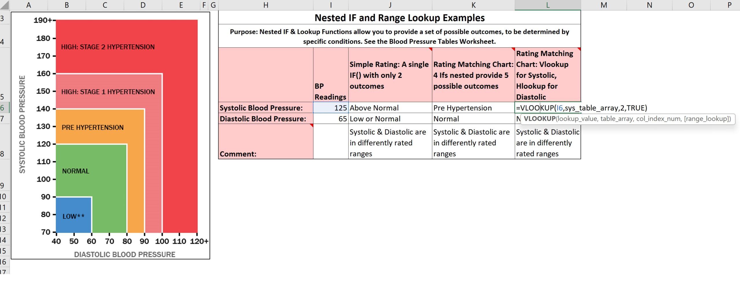
So, I’m going to adjust the page, to give the optimal view, and explain what we have here. We have a table that has a Systolic and a Diastolic blood pressure reading for some individual. And we’ve got an illustration here showing different ratings for different ranges of readings. So, for example, someone would be in the “low” range for a Systolic blood pressure reading if it was below 90. They would be in the “normal” range if it was below 120 and greater than or equal to 90. And so on. So, that is a situation where it’s very convenient to use a RANGE lookup to find the area that the reading falls in, because any reading, from 90 on up to just under 120 would be in the “normal” range, for example. So to
create a Table Array to emulate the same values that are in this illustration, we have a separate worksheet that has blood pressure tables.
And, we’ve got a vertical Table Array for the Systolic blood pressure readings. And we see that the top left corner is the lowest value possible. Which of course nobody would have a zero blood pressure reading, but that’s the lowest value to be categorized in the “low” range. 90 would be the lowest value to be categorized in the “normal” range, and we’ve named that range “Sys low normal.” 120 would be the lowest to be in the “pre-hypertension” range, and so on. So, the way a Vlookup() works with a RANGE lookup, the argument,
the first argument, to a Vlookup(), is the Lookup Value. The value that we want to look up in the table. And you can see here, with this Vlookup(), over here in cell L6,
I6 is the Lookup Value. And that is, in this case, the value 125. So we’re asking the Vlookup() Function to look up that value in the Table Array named Sys Table Array, and then return the value found in column 2 of that table,
once it settles on the RANGE that the reading falls within. And the TRUE argument, here, the 4th argument of the Vlookup(), is the RANGE Lookup argument, and when it’s TRUE, it means “Yes” this is a RANGE lookup. So the Vlookup() Function will take I6, the value 125, and it’ll go to the table array which is named
Sys Table Array, we can see it selected here. And it starts in the top left corner of the table, compares that value, that Lookup Value, to the value in that top left corner. If the value is greater than or equal to that value then it says, well this could be the right place, and then it goes on to the next one.It says, “Is 125 greater than or equal to this value?” Yes it is greater than or equal, so it says, this could be the right place. It goes on to the next one, “Is 125 greater than or equal to 120 in the pre-hypertension range?” and that’s true too, so then it goes to this one: “Is this greater, is it greater than or equal to 140?” No, so it’s NOT in this range. So, it goes back to this one, and it says, that this is the RANGE that we fall within. And now it’s going to return the value in column 2 of the table, in the same row as the value that the range identifies, so it’ll return the value “Pre-Hypertension.”
We could go back to that function, and we see that that is the result of this Vlookup(), was “Pre-Hypertension” for the value 125 and it’s a Vertical Lookup,
and the table is arranged vertically. Thank You.